The number of principal components. Application of principal component analysis to multivariate statistical data processing

Principal component analysis is a method that translates a large number of related (dependent, correlated) variables into fewer independent variables, since a large number of variables often complicates the analysis and interpretation of information. Strictly speaking, this method does not apply to factor analysis, although it has much in common with it. What is specific is, first, that in the course of computational procedures all principal components are simultaneously obtained and their number is initially equal to the number of initial variables; secondly, the possibility of a complete expansion of the variance of all initial variables is postulated, i.e. its full explanation through latent factors (generalized signs).

For example, suppose we conducted a study that measured students' intelligence on the Wechsler test, Eysenck test, Raven's test, and academic performance in social, cognitive, and general psychology. It is possible that the scores of various intelligence tests will correlate with each other, since they, after all, measure one characteristic of the test subject - his intellectual ability, although in different ways. If there are too many variables in the study ( x 1 , x 2 , …, x p ) , and some of them are interrelated, then the researcher sometimes has a desire to reduce the complexity of the data by reducing the number of variables. For this, the principal component method is used, which creates several new variables. y 1 , y 2 , …, y p , each of which is a linear combination of the original variables x 1 , x 2 , …, x p :

y 1 \u003d a 11 x 1 + a 12 x 2 +… + a 1p x p

y 2 \u003d a 21 x 1 + a 22 x 2 +… + a 2p x p

… (1)

y p \u003d a p1 x 1 + a p2 x 2 +… + a pp x p

Variables y 1 , y 2 , …, y p are called principal components or factors. Thus, a factor is an artificial statistical indicator that arises as a result of special transformations of the correlation matrix . The factor extraction procedure is called matrix factorization. As a result of factorization, a different number of factors can be extracted from the correlation matrix, up to a number equal to the number of initial variables. However, the factors determined as a result of factorization, as a rule, are not of equal importance.

Odds a ij defining a new variable are chosen so that the new variables (principal components, factors) describe the maximum amount of data variability and do not correlate with each other. It is often helpful to present odds a ij so that they represent the correlation coefficient between the original variable and the new variable (factor). This is achieved by multiplying a ij on the standard deviation of the factor. Most statistical packages do this (and STATISTICA too). Oddsa ij They are usually presented in the form of a table, where factors are arranged in columns, and variables in the form of rows:

Such a table is called a table (matrix) of factor loadings. The numbers given in it are the coefficients a ij The number 0.86 means that the correlation between the first factor and the value according to the Wechsler test is 0.86. The higher the factor load in absolute terms, the stronger the relationship between the variable and the factor.

Principal component method

Principal component method (eng. Principal component analysis, PCA ) is one of the main ways to reduce the dimension of data, losing the least amount of information. Invented by K. Pearson (eng. Karl pearson ) in d. It is used in many fields, such as pattern recognition, computer vision, data compression, etc. The calculation of the principal components is reduced to the calculation of eigenvectors and eigenvalues \u200b\u200bof the covariance matrix of the initial data. The principal component method is sometimes called karhunen-Loeve transformation (eng. Karhunen-loeve) or Hotelling transformation (eng. Hotelling transform). Other ways to reduce the dimension of data are the method of independent components, multidimensional scaling, as well as numerous nonlinear generalizations: the method of principal curves and manifolds, the method of elastic maps, finding the best projection (eng. Projection pursuit), neural network methods "bottleneck", etc.

Formal problem statement

The principal component analysis problem has at least four basic versions:

• approximate data with linear manifolds of lower dimension;
• find subspaces of lower dimension, in the orthogonal projection on which the spread of the data (that is, the standard deviation from the mean) is maximum;
• find subspaces of lower dimension, in the orthogonal projection to which the root-mean-square distance between points is maximum;
• for a given multidimensional random variable, construct such an orthogonal transformation of coordinates that, as a result of the correlation between individual coordinates, it will turn to zero.

The first three versions operate on finite data sets. They are equivalent and do not use any hypothesis about statistical data generation. The fourth version operates with random variables. Finite sets appear here as samples from a given distribution, and the solution of the first three problems as an approximation to the "true" Karhunen-Loeve transformation. This raises an additional and not completely trivial question about the accuracy of this approximation.

Fitting data with linear manifolds

Illustration for the famous work of K. Pearson (1901): given points on a plane, - the distance from to a straight line. Looking for a straight line that minimizes the amount

The principal component method began with the problem of the best approximation of a finite set of points by lines and planes (K. Pearson, 1901). A finite set of vectors is given. For each, among all -dimensional linear manifolds in, find such that the sum of the squares of the deviations from is minimal:

,

where is the Euclidean distance from a point to a linear manifold. Any -dimensional linear manifold in can be specified as a set of linear combinations, where the parameters run through the real line, and is an orthonormal set of vectors

,

where is the Euclidean norm, is the Euclidean scalar product, or in coordinate form:

.

The solution to the approximation problem for is given by a set of embedded linear manifolds,. These linear manifolds are defined by an orthonormal set of vectors (vectors of principal components) and a vector. The vector is sought as a solution to the minimization problem for:

.

Principal component vectors can be found as solutions to the same type of optimization problems:

1) centralize the data (subtract the average):. Now ; 2) find the first principal component as a solution to the problem; ... If the solution is not unique, then we choose one of them. 3) Subtract the projection onto the first main component from the data:; 4) find the second principal component as a solution to the problem. If the solution is not unique, then we choose one of them. … 2k-1) Subtract the projection onto the -th principal component (recall that the projections onto the previous principal components have already been subtracted):; 2k) find the k-th principal component as a solution to the problem:. If the solution is not unique, then we choose one of them. ...

At each preparatory step, subtract the projection onto the previous principal component. The found vectors are orthonormal simply as a result of solving the described optimization problem, however, in order to prevent computation errors from violating the mutual orthogonality of the vectors of the principal components, they can be included in the conditions of the optimization problem.

Non-uniqueness in the definition, apart from the trivial arbitrariness in the choice of the sign (and they solve the same problem), can be more essential and occur, for example, from the conditions of data symmetry. The last principal component is a unit vector orthogonal to all previous ones.

Finding Orthogonal Projections with the Most Scattering

The first principal component maximizes the sample variance of the data projection

Let's say we are given a centered set of data vectors (the arithmetic mean is zero). The task is to find such an orthogonal transformation to a new coordinate system, for which the following conditions would be true:

Singular value decomposition theory was created by J.J. Sylvester (eng. James joseph sylvester ) in G. and is presented in all the detailed manuals on matrix theory.

Simple iterative singular value decomposition algorithm

The main procedure is to find the best approximation of an arbitrary matrix by a matrix of the form (where is a -dimensional vector, and - is a -dimensional vector) by the least squares method:

The solution to this problem is given by successive iterations using explicit formulas. With a fixed vector, the values \u200b\u200bthat give the minimum to the form are uniquely and explicitly determined from the equalities:

Similarly, for a fixed vector, the values \u200b\u200bare determined:

As the initial approximation of the vector, we take a random vector of unit length, calculate the vector, then calculate the vector for this vector, etc. Each step decreases the value. As a stopping criterion, the smallness of the relative decrease in the value of the minimized functional per iteration step () or the smallness of the value itself is used.

As a result, the best approximation was obtained for the matrix by the matrix of the form (here the superscript denotes the approximation number). Further, we subtract the resulting matrix from the matrix, and for the obtained deviation matrix we again look for the best approximation of the same type, etc., until, for example, the norm becomes sufficiently small. As a result, we obtained an iterative procedure for decomposing a matrix in the form of a sum of matrices of rank 1, that is. We assume and normalize vectors: As a result, an approximation of singular numbers and singular vectors (right - and left -) is obtained.

The advantages of this algorithm include its exceptional simplicity and the ability to transfer it to data with spaces, as well as weighted data, almost unchanged.

There are various modifications to the basic algorithm to improve accuracy and stability. For example, the vectors of the principal components for different ones should be orthogonal "by construction", however, with a large number of iterations (large dimension, many components), small deviations from orthogonality accumulate and a special correction may be required at each step, ensuring its orthogonality to the previously found principal components.

Singular value decomposition and tensor principal component method

Often a data vector has the additional structure of a rectangular table (for example, a flat image) or even a multidimensional table - that is, a tensor:,. In this case, it is also effective to use the singular value decomposition. The definition, basic formulas and algorithms are carried over practically unchanged: instead of the data matrix, we have the -index value, where the first index is the number of the data point (tensor).

The main procedure is to find the best approximation of a tensor by a tensor of the form (where is the -dimensional vector (is the number of data points), is the vector of dimension at) by the least squares method:

The solution to this problem is given by successive iterations using explicit formulas. If all the vectors-factors are given except one, then this remaining one is determined explicitly from the sufficient minimum conditions.

As an initial approximation of vectors (), we take random vectors of unit length, calculate a vector, then for this vector and these vectors, calculate a vector, etc. (cyclically iterating over the indices) Each step decreases the value. The algorithm obviously converges. As a stopping criterion, the smallness of the relative decrease in the value of the minimized functional per cycle or the smallness of the value itself is used. Further, we subtract the obtained approximation from the tensor, and for the remainder we again seek the best approximation of the same type, etc., until, for example, the norm of the next remainder becomes sufficiently small.

This multicomponent singular value decomposition (tensor principal component method) is successfully used in the processing of images, video signals, and, more broadly, any data that has a tabular or tensor structure.

Conversion matrix to principal components

The transformation matrix of data to principal components consists of vectors of principal components, arranged in descending order of eigenvalues:

(means transpose),

That is, the matrix is \u200b\u200borthogonal.

Most of the data variation will be concentrated in the first coordinates, which allows you to move to a space of lower dimensions.

Residual variance

Let the data be centered,. When replacing data vectors with their projection onto the first principal components, the mean square of the error is introduced per one data vector:

where the eigenvalues \u200b\u200bof the empirical covariance matrix, arranged in descending order, taking into account the multiplicity.

This quantity is called residual variance... The quantity

called explained variance... Their sum is equal to the sample variance. The corresponding squared relative error is the ratio of residual variance to sample variance (i.e. proportion of unexplained variance):

By the relative error, the applicability of the principal component method with projection onto the first components is estimated.

Comment: in most computational algorithms, the eigenvalues \u200b\u200bwith the corresponding eigenvectors - the principal components are calculated in the order "from large to smallest". To calculate, it is enough to calculate the first eigenvalues \u200b\u200band the trace of the empirical covariance matrix, (the sum of the diagonal elements, that is, the variances along the axes). Then

Selection of principal components according to the Kaiser rule

The target approach to estimating the number of principal components based on the required fraction of the explained variance is formally always applicable, but implicitly it assumes that there is no separation into “signal” and “noise”, and any predetermined accuracy makes sense. Therefore, a different heuristic based on the hypothesis of the presence of a “signal” (relatively small dimension, relatively large amplitude) and “noise” (large dimension, relatively small amplitude) is often more productive. From this point of view, the principal component method works like a filter: the signal is contained mainly in the projection onto the first principal components, and in the remaining components the proportion of noise is much higher.

Question: how to estimate the number of required principal components if the signal-to-noise ratio is not known in advance?

The simplest and oldest method for selecting principal components gives kaiser's rule (eng. Kaiser "s rule): those main components are significant for which

that is, it exceeds the mean (mean sample variance of the coordinates of the data vector). The Kaiser rule works well in simple cases when there are several principal components with much higher than the mean, and the rest of the eigenvalues \u200b\u200bare less than it. In more complex cases, it can give too many significant principal components. If the data are normalized to a unit sample variance along the axes, then the Kaiser rule takes on an especially simple form: only those principal components are significant for which

Estimating the number of principal components by the broken cane rule

Example: Estimating the number of principal components by the broken cane rule in dimension 5.

One of the most popular heuristic approaches to estimating the number of principal components required is broken cane rule (eng. Broken stick model). The set of eigenvalues \u200b\u200bnormalized to the unit sum (,) is compared with the distribution of the lengths of the fragments of the reed of unit length broken at the th randomly selected point (the break points are chosen independently and are equally distributed along the length of the reed). Let () be the lengths of the obtained pieces of the cane, numbered in descending order of length:. It is not hard to find the mathematical expectation:

According to the broken cane rule, the th eigenvector (in descending eigenvalue order) is stored in the list of principal components if

In Fig. an example is given for the 5-dimensional case:

=(1+1/2+1/3+1/4+1/5)/5; =(1/2+1/3+1/4+1/5)/5; =(1/3+1/4+1/5)/5; =(1/4+1/5)/5; =(1/5)/5.

For example, selected

=0.5; =0.3; =0.1; =0.06; =0.04.

According to the broken cane rule, 2 main components should be left in this example:

According to user estimates, the broken cane rule tends to underestimate the number of significant principal components.

Normalization

Normalization after reduction to principal components

After of projection onto the first principal components with, it is convenient to normalize to the unit (sample) dispersion along the axes. The variance along the x principal component is equal to), therefore, for normalization, it is necessary to divide the corresponding coordinate by. This transformation is not orthogonal and does not preserve the dot product. The covariance matrix of the data projection after normalization becomes unit, the projections to any two orthogonal directions become independent values, and any orthonormal basis becomes the basis of the principal components (recall that normalization changes the vector orthogonality ratio). The mapping from the original data space to the first principal components, together with normalization, is given by the matrix

.

It is this transformation that is most often called the Karhunen-Loeve transformation. Here are column vectors and superscript means transpose.

Normalization before calculating principal components

Warning: one should not confuse the normalization carried out after the transformation to the main components with the normalization and "dimensionlessization" at data preprocessingcarried out before calculating the principal components. Pre-normalization is needed for a reasonable choice of the metric in which the best approximation of the data will be calculated, or the directions of the greatest scatter will be sought (which is equivalent). For example, if the data are three-dimensional vectors of "meters, liters and kilogram", then using the standard Euclidean distance, a difference of 1 meter in the first coordinate will make the same contribution as a difference of 1 liter in the second, or 1 kg in the third ... Usually, the systems of units in which the initial data are presented do not accurately reflect our ideas about the natural scales along the axes, and “dimensionlessness” is carried out: each coordinate is divided into a certain scale determined by the data, the purposes of their processing, and the measurement and data collection processes.

There are three essentially different standard approaches to such a normalization: unit variance along the axes (the scales along the axes are equal to the mean square deviations - after this transformation, the covariance matrix coincides with the matrix of correlation coefficients), on equal measurement accuracy (the scale along the axis is proportional to the measurement accuracy of this value) and on equal claims in the problem (the scale along the axis is determined by the required forecast accuracy of a given value or its permissible distortion - the level of tolerance). The choice of preprocessing is influenced by the meaningful formulation of the problem, as well as the conditions for data collection (for example, if the data collection is fundamentally incomplete and the data will still come, then it is irrational to choose the normalization strictly to unit variance, even if this corresponds to the meaning of the problem, since this implies the renormalization of all data after receiving a new portion; it is more reasonable to choose some scale that roughly estimates the standard deviation, and then not change it).

Pre-normalization to unit dispersion along the axes is destroyed by rotating the coordinate system if the axes are not principal components, and normalization during data preprocessing does not replace normalization after reduction to principal components.

Mechanical analogy and principal component analysis for weighted data

If we associate each data vector with a unit mass, then the empirical covariance matrix will coincide with the inertia tensor of this system of point masses (divided by the total mass), and the problem of principal components - with the problem of reducing the tensor of inertia to the principal axes. Additional freedom in the choice of mass values \u200b\u200bcan be used to account for the importance of data points or the reliability of their values \u200b\u200b(more masses are assigned to important data or data from more reliable sources). If the data vector is given mass, then instead of the empirical covariance matrix we get

All further operations to reduce to principal components are performed in the same way as in the basic version of the method: we look for an orthonormal eigenbasis, arrange it in descending order of eigenvalues, estimate the weighted average error of approximating the data by the first components (by the sums of eigenvalues), normalize, etc. ...

A more general weighing method gives maximizing the weighted sum of pairwise distances between projections. For every two data points, a weight is entered; and. Instead of the empirical covariance matrix, use

For, the symmetric matrix is \u200b\u200bpositive definite, since the quadratic form is positive:

Next, we look for an orthonormal proper basis, order it in descending order of eigenvalues, estimate the weighted average error of approximating the data by the first components, etc. - exactly as in the main algorithm.

This method is applied if there are classes: for different classes, the weight is chosen to be larger than for points of the same class. As a result, in the projection onto the weighed principal components, different classes are "moved apart" to a greater distance.

Another application is reducing the influence of large deviations (outlays, eng. Outlier ), which can distort the picture due to the use of the rms distance: if selected, the effect of large deviations will be reduced. Thus, the described modification of the principal component method is more robust than the classical one.

Special terminology

In statistics, when using the principal component analysis, several technical terms are used.

Data matrix ; each row is a vector pre-processed data ( centered and right normalized), number of rows - (number of data vectors), number of columns - (dimension of data space);

Load matrix (Loadings); each column is a vector of principal components, the number of rows is (dimension of the data space), the number of columns is (the number of vectors of principal components selected for projection);

Account Matrix (Scores); each row is the projection of the data vector onto the principal components; number of rows - (number of data vectors), number of columns - (number of principal component vectors selected for projection);

Z-score matrix (Z-scores); each row is the projection of the data vector onto the principal components, normalized to the unit sample variance; number of rows - (number of data vectors), number of columns - (number of principal component vectors selected for projection);

Error matrix (or leftovers) (Errors or residuals).

Basic formula:

Limits of applicability and limitations of the effectiveness of the method

Principal component analysis is always applicable. The widespread statement that it is applicable only to normally distributed data (or for distributions close to normal) is incorrect: in the original formulation of K. Pearson, the problem is posed about approximations a finite set of data, and there is not even a hypothesis about their statistical generation, not to mention the distribution.

However, the method does not always effectively reduce the dimension under the given accuracy constraints. Lines and planes do not always provide a good approximation. For example, the data can follow a curve with good accuracy, and that curve can be difficult to position in the data space. In this case, the principal component analysis will require several components (instead of one) for acceptable accuracy, or will not give a reduction in dimension at all with acceptable accuracy. To work with such "curves" of principal components, the method of principal manifolds and various versions of the nonlinear method of principal components were invented. Data with complex topology can cause more trouble. Various methods have also been invented to approximate them, such as self-organizing Kohonen maps, neural gas, or topological grammars. If the data is statistically generated with a distribution that is very different from the normal, then to approximate the distribution it is useful to go from the principal components to independent components that are no longer orthogonal in the original dot product. Finally, for an isotropic distribution (even normal), instead of a scattering ellipsoid, we obtain a ball, and it is impossible to reduce the dimension by approximation methods.

Examples of using

Data visualization

Data visualization - the presentation in a visual form of experimental data or the results of a theoretical study.

The first choice in visualizing a dataset is to orthogonal projection onto the plane of the first two principal components (or the 3-dimensional space of the first three principal components). The design plane is essentially a flat, two-dimensional "screen" positioned to provide a "picture" of the data with the least amount of distortion. Such a projection will be optimal (among all orthogonal projections onto different two-dimensional screens) in three respects:

1. The minimum sum of squared distances from data points to projections onto the plane of the first principal components, that is, the screen is located as close as possible to the point cloud.
2. The minimum amount of distortion of the squares of the distances between all pairs of points from the data cloud after the projection of the points on the plane.
3. Minimum sum of distortions of squared distances between all data points and their "center of gravity".

Data visualization is one of the most widely used applications of principal component analysis and its nonlinear generalizations.

Compression of images and videos

To reduce the spatial redundancy of pixels when coding images and video, linear transformations of blocks of pixels are used. Subsequent quantization of the obtained coefficients and lossless coding allow obtaining significant compression ratios. Using the PCA transform as a linear transform is optimal for some types of data in terms of the size of the obtained data with the same distortion. At the moment, this method is not actively used, mainly due to the great computational complexity. Also, data compression can be achieved by discarding the last conversion factors.

Reducing noise in images

Chemometrics

Principal component analysis is one of the main methods in chemometrics (eng. Chemometrics ). Allows to divide the matrix of the initial data X into two parts: "meaningful" and "noise". By the most popular definition, "Chemometrics is a chemical discipline that uses mathematical, statistical and other methods based on formal logic to construct or select optimal measurement methods and experimental designs, and to extract the most important information in the analysis of experimental data."

Psychodiagnostics

1. data analysis (description of the results of surveys or other studies, presented in the form of arrays of numerical data);
2. description of social phenomena (construction of models of phenomena, including mathematical models).

In political science, the principal component method was the main tool of the Political Atlas of Modernity project for linear and nonlinear analysis of the ratings of 192 countries of the world according to five specially developed integral indices (living standards, international influence, threats, statehood and democracy). For the cartography of the results of this analysis, a special GIS (Geographic Information System) has been developed that combines the geographic space with the space of features. Political atlas data maps have also been created using the two-dimensional principal manifolds in the five-dimensional space of countries as a substrate. The difference between a data map and a geographic map is that on a geographic map there are objects that have similar geographic coordinates nearby, while on a data map there are objects (countries) with similar attributes (indices) nearby.

The data matrix is \u200b\u200bthe source for the analysis

dimensions
, the i-th row of which characterizes the i-th observation (object) for all k indicators
... Initial data are normalized, for which the average values \u200b\u200bof indicators are calculated
, as well as the values \u200b\u200bof standard deviations
... Then the matrix of normalized values

with elements

The matrix of paired correlation coefficients is calculated:

The main diagonal of the matrix contains the unit elements
.

The component analysis model is built by presenting the original normalized data as a linear combination of the principal components:

where - "weight", i.e. factor loading th main component on th variable;

-value th main component for -th observation (object), where
.

In matrix form, the model has the form

here
- matrix of principal components of dimension
,

- matrix of factorial loads of the same dimension.

Matrix
describes observations in space main components. Moreover, the elements of the matrix
are normalized, and the principal components are not correlated with each other. It follows that
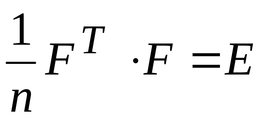where - unit matrix of dimension
.

Element matrices characterizes the tightness of the linear relationship between the original variable and the main component , therefore, takes the values
.

Correlation matrix can be expressed in terms of factor loadings matrix .

Units are located along the main diagonal of the correlation matrix and, by analogy with the covariance matrix, they represent the variances of the used - features, but unlike the latter, due to normalization, these variances are equal to 1. The total variance of the entire system - features in the sample volume
is equal to the sum of these units, i.e. is equal to the trace of the correlation matrix
.

The correlation matrix can be converted to a diagonal matrix, that is, a matrix, all values \u200b\u200bof which, except for the diagonal ones, are equal to zero:

,

where
- a diagonal matrix, on the main diagonal of which there are eigenvalues correlation matrix, is a matrix whose columns are the eigenvectors of the correlation matrix ... Since the matrix R is positive definite, i.e. its major minors are positive, then all eigenvalues
for any
.

Eigenvalues are found as the roots of the characteristic equation

Eigenvector corresponding to the eigenvalue correlation matrix , is defined as a nonzero solution to the equation

Normalized eigenvector is equal

The vanishing of the off-diagonal terms means that the features become independent of each other (
at
).

Total variance of the entire system variables in the sample remains the same. However, its values \u200b\u200bare redistributed. The procedure for finding the values \u200b\u200bof these variances is to find the eigenvalues correlation matrix for each of - signs. The sum of these eigenvalues
is equal to the trace of the correlation matrix, i.e.
, that is, the number of variables. These eigenvalues \u200b\u200bare the variance values \u200b\u200bof the features
in conditions if the signs were independent of each other.

In the method of principal components, the correlation matrix is \u200b\u200bfirst calculated from the initial data. Then, its orthogonal transformation is performed and through this factor loadings are found for all variables and
factors (factor load matrix), eigenvalues and determine the weights of the factors.

The factor loadings matrix A can be defined as
, and -th column of matrix A - as
.

Weight of factors
or
reflects the share in the total variance introduced by this factor.

Factor loadings vary from –1 to +1 and are analogous to the correlation coefficients. In the matrix of factor loads, it is necessary to select significant and insignificant loads using the Student's t test
.

Sum of squares of loads th factor in all - signs is equal to the eigenvalue of this factor
... Then
- the contribution of the i-th variable in% to the formation of the j-th factor.

The sum of the squares of all factorial loads in a row is equal to one, the total variance of one variable, and all factors for all variables is equal to the total variance (i.e., the trace or order of the correlation matrix, or the sum of its eigenvalues)
.

In general, the factorial structure of the i-th feature is presented in the form
, which includes only significant loads. Using the factorial loadings matrix, it is possible to calculate the values \u200b\u200bof all factors for each observation of the original sample population by the formula:

,

where - the value of the j-th factor in the t-th observation, -standardized value of the i-th feature in the t-th observation of the original sample; –Factor load, –The intrinsic value corresponding to the factor j. These calculated values are widely used for graphical presentation of the results of factor analysis.

The correlation matrix can be restored from the factor loadings matrix:
.

The part of the variance of a variable explained by the principal components is called the generality.

,

where is the variable number, and -number of the main component. The correlation coefficients reconstructed only for the main components will be less than the original ones in absolute value, and on the diagonal there will be not 1, but the values \u200b\u200bof the communities.

Specific contribution -th main component is determined by the formula

.

The total contribution of the
principal components are determined from the expression

.

Usually used for analysis
the first principal components, whose contribution to the total variance exceeds 60-70%.

The factor loadings matrix A is used for the interpretation of principal components, while those values \u200b\u200bare usually considered that exceed 0.5.

Principal component values \u200b\u200bare given by the matrix

In an effort to accurately describe the area of \u200b\u200binterest, analysts often select a large number of independent variables (p). In this case, a serious error can occur: several descriptive variables can characterize the same side of the dependent variable and, as a result, highly correlate with each other. The multicollinearity of the independent variables seriously distorts the research results, so it should be avoided.

Principal component analysis (as a simplified factor analysis model, since this method does not use individual factors describing only one variable x i) allows you to combine the influence of highly correlated variables into one factor characterizing the dependent variable from one side. As a result of the analysis carried out by the method of principal components, we will achieve the compression of information to the required size, the description of the dependent variable m (m

First, you need to decide how many factors you need to highlight in this study. Within the framework of the method of principal components, the first main factor describes the largest percentage of variance of independent variables, then - in decreasing order. Thus, each successive main component, identified sequentially, explains a smaller proportion of the variability of factors x i. The challenge for the researcher is to determine when the variability becomes truly small and random. In other words, how many principal components should be selected for further analysis.

There are several methods for the rational selection of the required number of factors. The most used of these is the Kaiser test. According to this criterion, only those factors are selected whose eigenvalues \u200b\u200bare greater than 1. Thus, a factor that does not explain the variance equivalent to at least the variance of one variable is omitted.

Let's analyze Table 19 built in SPSS:

Table 19. Total variance explained

Component	Initial eigenvalues	Sums of squares of rotational loads
Total	% Dispersion	Cumulative%	Total	% Dispersion	Cumulative%
dimension0		5,442	90,700	90,700	3,315	55,246	55,246
	,457	7,616	98,316	2,304	38,396	93,641
	,082	1,372	99,688	,360	6,005	99,646
	,009	,153	99,841	,011	,176	99,823
	,007	,115	99,956	,006	,107	99,930
	,003	,044	100,000	,004	,070	100,000
Isolation method: Principal component analysis.

As can be seen from Table 19, in this study, the xi variables are highly correlated with each other (this was also revealed earlier and can be seen from Table 5 "Pairwise correlation coefficients"), and therefore, characterize the dependent variable Y practically from one side: initially, the first principal component explains 90 , 7% of the variance xi, and only the eigenvalue corresponding to the first principal component is greater than 1. Of course, this is a drawback of data selection, but in the selection process this drawback was not obvious.

Analysis in the SPSS package allows you to independently select the number of principal components. Let's choose the number 6 - equal to the number of independent variables. The second column of Table 19 shows the sum of the squares of the rotational loads, and it is from these results that we draw a conclusion about the number of factors. The eigenvalues \u200b\u200bcorresponding to the first two principal components are greater than 1 (55.246% and 38.396%, respectively), therefore, according to the Kaiser method, we will single out the 2 most significant principal components.

The second method for identifying the required number of factors is the “scree” criterion. According to this method, the eigenvalues \u200b\u200bare presented in the form of a simple graph, and a place on the graph is selected where the decrease of the eigenvalues \u200b\u200bfrom left to right slows down as much as possible:

Figure 3. Scree criterion

As can be seen in Figure 3, the decay of the eigenvalues \u200b\u200bslows down from the second component, but the constant rate of decay (very small) starts only from the third component. Therefore, the first two principal components will be selected for further analysis. This conclusion is consistent with the conclusion obtained using the Kaiser method. Thus, the first two successively obtained principal components are finally selected.

After identifying the main components that will be used in further analysis, it is necessary to determine the correlation of the initial variables x i with the obtained factors and, based on this, give names to the components. For the analysis, we will use the factor loadings matrix A, the elements of which are the coefficients of the correlation of factors with the original independent variables:

Table 20. Factor loadings matrix

Component matrix a
	Component
X1	,956	-,273	,084	,037	-,049	,015
X2	,986	-,138	,035	-,080	,006	,013
X3	,963	-,260	,034	,031	,060	-,010
X4	,977	,203	,052	-,009	-,023	-,040
X5	,966	,016	-,258	,008	-,008	,002
X6	,861	,504	,060	,018	,016	,023
Isolation method: Principal component analysis.
a. Extracted components: 6

In this case, the interpretation of the correlation coefficients is difficult, therefore, it is rather difficult to name the first two main components. Therefore, we will further use the Varimax method of orthogonal rotation of the coordinate system, the purpose of which is to rotate the factors so as to choose the simplest factor structure for interpretation:

Table 21. Coefficients of interpretation

Rotated component matrix a
	Component
X1	,911	,384	,137	-,021	,055	,015
X2	,841	,498	,190	,097	,000	,007
X3	,900	,390	,183	-,016	-,058	-,002
X4	,622	,761	,174	,022	,009	,060
X5	,678	,564	,472	,007	,001	,005
X6	,348	,927	,139	,001	-,004	-,016
Isolation method: Principal component analysis. Rotation method: Varimax with Kaiser normalization.
a. The rotation converged in 4 iterations.

From Table 21 it can be seen that the first principal component is most associated with the variables x1, x2, x3; and the second one with variables x4, x5, x6. Thus, we can conclude that investment in fixed assets in the region (variable Y) depends on two factors:

- the volume of own and borrowed funds received by the enterprises of the region for the period (first component, z1);

- as well as the intensity of investments by regional enterprises in financial assets and the amount of foreign capital in the region (second component, z2).

Figure 4. Scatter diagram

This diagram shows disappointing results. At the very beginning of the study, we tried to select the data so that the resulting variable Y was distributed normally, and we practically succeeded. The distribution laws of the independent variables were quite far from normal, but we tried to bring them as close as possible to the normal law (to select the data accordingly). Figure 4 shows that the initial hypothesis about the closeness of the distribution law of independent variables to the normal law is not confirmed: the shape of the cloud should resemble an ellipse, in the center the objects should be located more densely than at the edges. It is worth noting that making a multidimensional sample, in which all variables are distributed according to the normal law, is a task that can be performed with great difficulty (moreover, it does not always have a solution). However, this goal should be pursued: then the results of the analysis will be more meaningful and understandable for interpretation. Unfortunately, in our case, when most of the work on analyzing the collected data has been done, it is rather difficult to change the sample. But further, in subsequent works, it is worth taking a more serious approach in the sample of independent variables and maximally approximating the law of their distribution to normal.

The last stage of the principal component analysis is the construction of a regression equation for the principal components (in this case, for the first and second principal components).

Using SPSS, we calculate the parameters of the regression model:

Table 22. Parameters of the regression equation for principal components

Model	Unstandardized odds	Standardized odds	t	Znch.
B	Std. Error	Beta
	(Constant)	47414,184	1354,505		35,005	,001
Z1	26940,937	1366,763	,916	19,711	,001
Z2	6267,159	1366,763	,213	4,585	,001

The regression equation will take the form:

y \u003d 47 414.184 + 0.916 * z1 + 0.213 * z2,

(b0) (b1) (b2)

t. about. b0=47 414,184 shows the point of intersection of the regression line with the axis of the resulting indicator;

b1 \u003d 0.916 -with an increase in the value of the factor z1 by 1, the expected average value of the amount of investment in fixed assets will increase by 0.916;

b2 \u003d 0.213 -with an increase in the value of the factor z2 by 1, the expected average value of the amount of investment in fixed assets will increase by 0.213.

In this case, the value of tcr ("alpha" \u003d 0.001, "nu" \u003d 53) \u003d 3.46 is less than tobl for all "beta" coefficients. Therefore, all coefficients are significant.

Table 24. Quality of the regression model for principal components

Model	R	R-square	Adjusted R-squared	Std. estimation error
dimension0		, 941 a	,885	,881	10136,18468
a. Predictors: (const) Z1, Z2
b. Dependent Variable: Y

Table 24 reflects indicators that characterize the quality of the constructed model, namely: R - multiple k-t correlation - indicates what proportion of the variance Y is explained by the variation in Z; R ^ 2 - to-t determination - shows the proportion of the explained variance of deviations of Y from its mean value. The standard error of the estimate characterizes the error of the constructed model. Let's compare these indicators with similar indicators of the power-law regression model (its quality turned out to be higher than the quality of the linear model, so we compare it with the power-law model):

Table 25. Quality of power regression model

So, multiple k-t correlation R and k-t determination R ^ 2 in the power model is slightly higher than in the principal component model. In addition, the standard error of the principal component model is MUCH higher than that of the power law. Therefore, the quality of a power-law regression model is higher than a regression model based on principal components.

Let us verify the regression model of the main components, i.e., analyze its significance. Let's check the hypothesis about the insignificance of the model, calculate F (obs.) \u003d 204.784 (calculated in SPSS), F (crit) (0.001; 2; 53) \u003d 7.76. F (obs)\u003e F (crit), therefore, the hypothesis that the model is insignificant is rejected. The model is meaningful.

So, as a result of the component analysis, it was found that from the selected independent variables xi, 2 main components can be distinguished - z1 and z2, and z1 is more influenced by the variables x1, x2, x3, and z2 - x4, x5, x6 ... The regression equation based on the principal components turned out to be significant, although it is inferior in quality to the power regression equation. According to the regression equation for principal components, Y positively depends on both Z1 and Z2. However, the initial multicollinearity of the variables xi and the fact that they are not distributed according to the normal distribution law can distort the results of the constructed model and make it less significant.

Cluster Analysis

The next stage of this research is cluster analysis. The task of cluster analysis is to divide the selected regions (n \u200b\u200b\u003d 56) into a relatively small number of groups (clusters) based on their natural proximity with respect to the values \u200b\u200bof the variables x i. When conducting cluster analysis, we assume that the geometric proximity of two or more points in space means the physical proximity of the corresponding objects, their homogeneity (in our case, the homogeneity of regions in terms of indicators affecting investments in fixed assets).

At the first stage of cluster analysis, it is necessary to determine the optimal number of allocated clusters. To do this, it is necessary to carry out hierarchical clustering - the sequential combination of objects into clusters until there are two large clusters, which are combined into one at the maximum distance from each other. The result of hierarchical analysis (conclusion about the optimal number of clusters) depends on the method of calculating the distance between clusters. Thus, we will test various methods and draw appropriate conclusions.

Nearest Neighbor Method

If we calculate the distance between individual objects in a unified way - as a simple Euclidean distance - the distance between clusters is calculated by different methods. According to the "nearest neighbor" method, the distance between clusters corresponds to the minimum distance between two objects of different clusters.

The analysis in the SPSS package is as follows. First, the matrix of distances between all objects is calculated, and then, based on the matrix of distances, the objects are sequentially combined into clusters (for each step, the matrix is \u200b\u200bcompiled anew). The steps for sequential combining are presented in the table:

Table 26. Steps of agglomeration. Nearest Neighbor Method

Stage	The cluster is merged with	Odds		Next stage
Cluster 1	Cluster 2	Cluster 1	Cluster 2
			,003
			,004
			,004
			,005
			,005
			,005
			,005
			,006
			,007
			,007
			,009
			,010
			,010
			,010
			,010
			,011
			,012
			,012
			,012
			,012
			,012
			,013
			,014
			,014
			,014
			,014
			,015
			,015
			,016
			,017
			,018
			,018
			,019
			,019
			,020
			,021
			,021
			,022
			,024
			,025
			,027
			,030
			,033
			,034
			,042
			,052
			,074
			,101
			,103
			,126
			,163
			,198
			,208
			,583
			1,072

As can be seen from Table 26, at the first stage, elements 7 and 8 were combined, since the distance between them was minimal - 0.003. Further, the distance between the combined objects increases. The table also shows the optimal number of clusters. To do this, you need to look after which step there is a sharp jump in the distance, and subtract the number of this agglomeration from the number of objects under study. In our case: (56-53) \u003d 3 is the optimal number of clusters.

Figure 5. Dendrogram. Nearest Neighbor Method

A similar conclusion about the optimal number of clusters can be made by looking at the dendrogram (Fig. 5): you should select 3 clusters, and the first cluster will include objects numbered 1-54 (54 objects in total), and the second and third clusters - one object each (numbered 55 and 56, respectively). This result suggests that the first 54 regions are relatively homogeneous in terms of indicators affecting investments in fixed assets, while objects numbered 55 (Republic of Dagestan) and 56 (Novosibirsk region) stand out significantly against the general background. It is worth noting that these entities have the largest investment in fixed assets among all selected regions. This fact once again proves the high dependence of the resulting variable (investment volume) on the selected independent variables.

Similar reasoning is carried out for other methods of calculating the distance between clusters.

Distant Neighbor Method

Table 27. Agglomeration steps. Distant Neighbor Method

Stage	The cluster is merged with	Odds	Stage of the first appearance of the cluster	Next stage
Cluster 1	Cluster 2	Cluster 1	Cluster 2
			,003
			,004
			,004
			,005
			,005
			,005
			,005
			,007
			,009
			,010
			,010
			,011
			,011
			,012
			,012
			,014
			,014
			,014
			,017
			,017
			,018
			,018
			,019
			,021
			,022
			,026
			,026
			,027
			,034
			,035
			,035
			,037
			,037
			,042
			,044
			,046
			,063
			,077
			,082
			,101
			,105
			,117
			,126
			,134
			,142
			,187
			,265
			,269
			,275
			,439
			,504
			,794
			,902
			1,673
			2,449

In the far neighbor method, the distance between clusters is calculated as the maximum distance between two objects in two different clusters. According to Table 27, the optimal number of clusters is (56-53) \u003d 3.

Figure 6. Dendrogram. Distant Neighbor Method

According to the dendrogram, the optimal solution would also be to select 3 clusters: the first cluster will include regions numbered 1-50 (50 regions), the second - 51-55 (5 regions), and the third - the last region numbered 56.

Center of gravity method

In the method of "center of gravity" the distance between clusters is the Euclidean distance between the "centers of gravity" of clusters - the arithmetic mean of their indices x i.

Figure 7. Dendrogram. Center of gravity method

Figure 7 shows that the optimal number of clusters is as follows: 1 cluster - 1-47 objects; 2 cluster - 48-54 objects (6 in total); Cluster 3 - 55 objects; 4 cluster - 56 objects.

Medium bond principle

In this case, the distance between clusters is equal to the average value of the distances between all possible pairs of observations, with one observation taken from one cluster, and the second, respectively, from the other.

Analysis of the agglomeration steps table showed that the optimal number of clusters is (56-52) \u003d 4. Let us compare this conclusion with the conclusion obtained from the analysis of the dendrogram. Figure 8 shows that cluster 1 will include objects numbered 1-50, cluster 2 - objects 51-54 (4 objects), cluster 3 - region 55, cluster 4 - region 56.

Figure 8. Dendrogram. Medium bond method

Component analysis refers to multidimensional dimensionality reduction techniques. It contains one method - the principal component method. Principal components represent an orthogonal coordinate system in which the component variances characterize their statistical properties.

Considering that the objects of research in the economy are characterized by a large, but finite number of features, the influence of which is influenced by a large number of random causes.

Calculation of principal components

The first main component Z1 of the studied system of features X1, X2, X3, X4, ..., Xn is called such a centered - a normalized linear combination of these features, which, among others, is centered - normalized linear combinations of these features, has the most variable variance.

As the second principal component Z2, we will take such a centered - normalized combination of these features, which:

not correlated with the first principal component,

not correlated with the first principal component, this combination has the highest variance.

The K-th principal component Zk (k \u003d 1 ... m) we will call such a centered - normalized combination of features, which:

not correlated with k-1 previous principal components,

among all possible combinations of initial features that are not

not correlated with the k-1 previous principal components, this combination has the highest variance.

We introduce an orthogonal matrix U and pass from variables X to variables Z, and

The vector is chosen so that the variance is maximal. After obtaining, it is chosen so that the variance is maximum, provided that it is not correlated with, etc.

Since the features are measured in incomparable quantities, it will be more convenient to switch to centered-normalized values. We find the matrix of the initial centered-normalized values \u200b\u200bof the features from the ratio:

where is an unbiased, consistent and effective estimate of the mathematical expectation,

Unbiased, consistent and efficient variance estimate.

The matrix of observed values \u200b\u200bof the initial features is given in the Appendix.

Centering and standardization was performed using the "Stadia" software.

Since the features are centered and normalized, the correlation matrix can be estimated using the formula:

Before carrying out the component analysis, let us analyze the independence of the initial characteristics.

Checking the significance of the pairwise correlation matrix using the Wilkes test.

We put forward a hypothesis:

H0: insignificant

H1: significant

125,7; (0,05;3,3) = 7,8

since k\u003e, then the hypothesis Н0 is rejected and the matrix is \u200b\u200bsignificant, therefore, it makes sense to carry out component analysis.

Let us check the conjecture about the diagonality of the covariance matrix

We put forward a hypothesis:

We build statistics, distributed according to the law with degrees of freedom.

123,21, (0,05;10) =18,307

since\u003e, then the hypothesis Н0 is rejected and it makes sense to carry out component analysis.

To construct a matrix of factor loads, it is necessary to find the eigenvalues \u200b\u200bof the matrix by solving the equation.

For this operation, we use the eigenvals function of the MathCAD system, which returns the eigenvalues \u200b\u200bof a matrix:

Because the initial data represent a sample from the general population, then we received not the eigenvalues \u200b\u200band eigenvectors of the matrix, but their estimates. We will be interested in how “good”, from a statistical point of view, the sample characteristics describe the corresponding parameters for the general population.

The confidence interval for the i-th eigenvalue is found by the formula:

The confidence intervals for the eigenvalues \u200b\u200bultimately take the form:

The estimate of the value of several eigenvalues \u200b\u200bfalls within the confidence interval of other eigenvalues. It is necessary to test the hypothesis about the multiplicity of the eigenvalues.

The cardinality is checked using statistics

where r is the number of multiple roots.

This statistic in the case of fairness is distributed according to the law with the number of degrees of freedom. Let's put forward hypotheses:

Since, the hypothesis is rejected, that is, the eigenvalues \u200b\u200bare not multiple.

Since, the hypothesis is rejected, that is, the eigenvalues \u200b\u200bare not multiple.

It is necessary to highlight the main components at the level of information content 0.85. The measure of informativeness shows what part or what proportion of the variance of the initial features are the k-first principal components. The measure of informativeness is the value:

At a given level of information content, three main components are identified.

We write the matrix \u003d

To obtain a normalized transition vector from the original features to the main components, it is necessary to solve the system of equations:, where is the corresponding eigenvalue. After obtaining a solution to the system, it is then necessary to normalize the resulting vector.

To solve this problem, we will use the eigenvec function of the MathCAD system, which returns the normalized vector for the corresponding eigenvalue.

In our case, the first four principal components are sufficient to achieve a given level of information content; therefore, the matrix U (the matrix of the transition from the initial basis to the basis of eigenvectors)

We construct a matrix U, whose columns are eigenvectors:

Weighting matrix:

The coefficients of the matrix A are the coefficients of correlation between the centered - normalized initial features and non-normalized principal components, and show the presence, strength and direction of the linear relationship between the corresponding initial features and the corresponding principal components.